Project - Finding Replacement Players in the Transfer Market using K-means Cluster Analysis in R

TL;DR

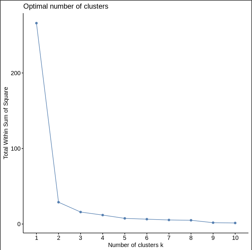
By using K-means cluster analysis in R, I was able to identify potential young replacements for aging Premier League players (Giroud, Fernandinho, and Vardy). By applying K-means clustering to my filtered dataset of players born after 1997 in the same positions, I created statistical groupings based on Goals+Assists and Expected Goals+Assists metrics. The K-means algorithm effectively separated players into distinct performance clusters, revealing which young talents most closely match the statistical profiles of these veterans. My data-mining approach determined the optimal number of clusters (2) for each position group, creating visual representations that clearly highlighted promising replacement candidates with similar performance characteristics to the established players.

Prerequisites & Packages

R Packages

readr

tidyr

ggplot2

dplyr

ggpubr

factoextra

readxl

stats

ggfortify

mclust

Considerations & Limitations

My K-means clustering analysis faced several constraints. Using only G+A and xG+A metrics provided a limited view of player performance, especially for defensive players like Fernandinho. The dataset lacked defensive statistics, biasing the analysis toward attacking contributions. Using just two clustering variables created simplistic groupings, while the freely accessible FBRef data lacked the granularity of professional datasets like Statsbomb.com. In future analyses, I would incorporate position-specific metrics and multiple clustering variables to reveal more nuanced statistical relationships and strengthen replacement recommendations. Additionally, including psychological and contextual data would better predict player adaptation to new environments, as statistical similarities alone are insufficient for predicting transfer success.

Step 1

Using R, install the required packages. The main ones being stats for the K-means clustering algorithm & factoextra / ggplot2 for clustering visualisation


# Install packages (run once)
install.packages(c("readr", "tidyr", "ggplot2", "dplyr", "ggpubr", 
                  "factoextra", "readxl", "stats", "ggfortify", "mclust"))

# Load packages
library(readr)
library(tidyr)
library(ggplot2)
library(dplyr)
library(ggpubr)
library(factoextra)
library(readxl)
library(stats)
library(ggfortify)
library(mclust)

Step 2

Import Data

 
# Read player data from Excel/CSV file
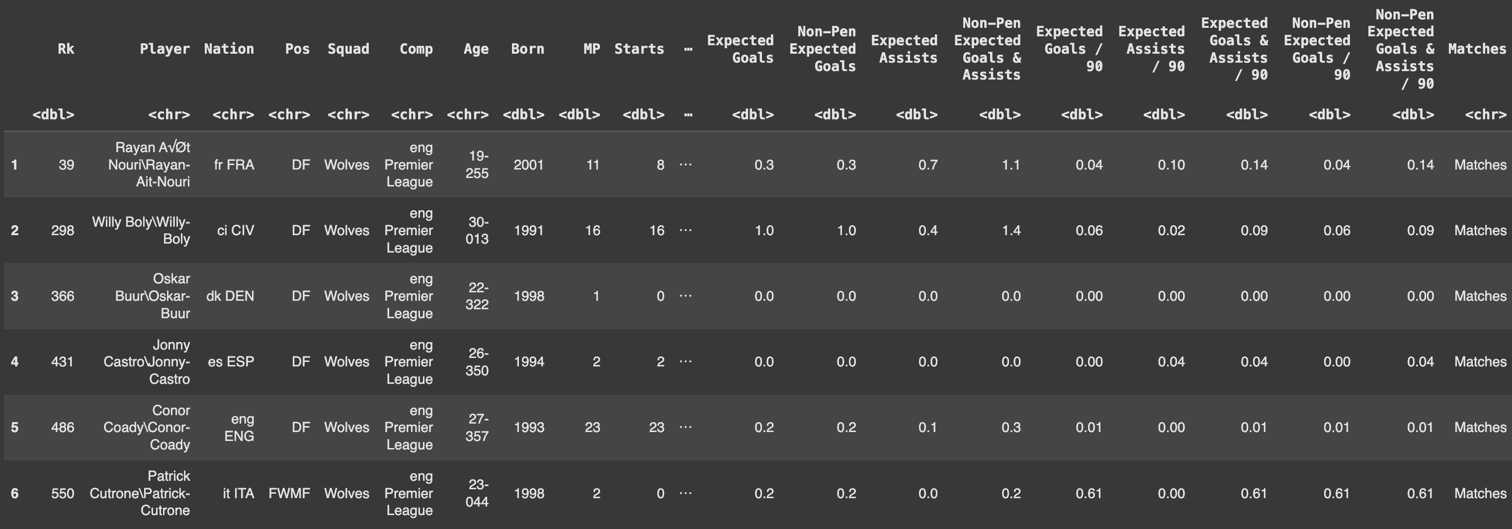
player_data <- read_excel("/content/FootballPlayerDataBase.xlsx", skip = 1)

# Convert to data frame
player_data <- as.data.frame(player_data)

K-means Cluster Analysis Visualization — Figure 1: Data Preview

Step 3

Filter Data for Each Player Analysis

 
# Example for Giroud replacement (Chelsea forward)
giroud_replacement <- player_data %>%
  filter((Pos == "FW" & Born > 1997) | Rk == "909")

# Example for Fernandinho replacement (Man City midfielder)
fernandinho_replacement <- player_data %>%
  filter((Pos == "MD" & Born > 1997) | Rk == "806")

# Example for Vardy replacement (Leicester forward)
vardy_replacement <- player_data %>%
  filter((Pos == "FW" & Born > 1997) | Rk == "2469")

Step 4

Clean the Data

 
#Remove NA values and clean data structure
giroud_clean <- na.omit(giroud_replacement)
giroud_clean <- as.data.frame(giroud_clean)

fernandinho_clean <- na.omit(fernandinho_replacement)
fernandinho_clean <- as.data.frame(fernandinho_clean)

vardy_clean <- na.omit(vardy_replacement)
vardy_clean <- as.data.frame(vardy_clean)

Step 5

Select Variables for Analysis


# For Giroud analysis (example)
giroud_vars <- giroud_clean %>%
  select(Player, `Goal & Assist / 90`, `Expected Goals & Assists / 90`)

Step 6

Determine Optimal Number of Clusters


# Set seed for reproducibility
set.seed(123)

# Find optimal number of clusters
fviz_nbclust(giroud_vars %>% select(-Player), kmeans, method = "wss")

Step 7

Perform K-means Cluster Analysis

 
# Using 2 clusters based on optimal number found
km_giroud <- kmeans(giroud_vars %>% select(-Player), centers = 2)

# Visualize the clusters
fviz_cluster(km_giroud, data = giroud_vars %>% select(-Player),
             palette = "jco",
             geom = "point",
             ellipse.type = "convex")

Step 8

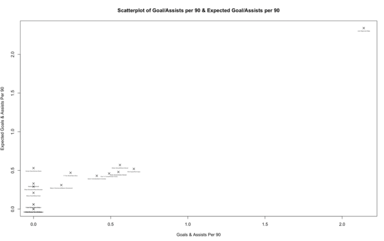
Create Labeled Scatter Plot for Player Identification

 
# Create scatter plot with player names
ggplot(giroud_vars, aes(x = `Goal & Assist / 90`, y = `Expected Goals & Assists / 90`)) +
  geom_point() +
  geom_text(aes(label = Player), vjust = 1.5, size = 3) +
  labs(title = "Potential Giroud Replacements",
       x = "Goals + Assists",
       y = "Expected Goals + Expected Assists") +
  theme_minimal()

Step 9

Repeat Steps 5-8 for Each Player

Step 10

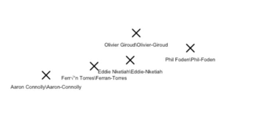
Analysis of Results -> Olivier Giroud

The K-means cluster analysis identified three potential replacements for Olivier Giroud: Phil Foden, Ferran Torres, and Eddie Nketiah.

Giroud's current statistical profile shows 0.56 G+A/90 and 0.57 xG+xA/90. Each replacement candidate offers different strengths:

Phil Foden (Manchester City): Shows higher G+A/90 at 0.65 but slightly lower xG+xA/90 at 0.52, suggesting potential overachievement this season. His versatility across attacking positions is valuable.

Ferran Torres (Manchester City): With 0.49 G+A/90 and 0.46 xG+xA/90, Torres scores slightly below Giroud but represents one of the closest statistical matches in the dataset. His age and potential for growth offset current statistical gaps.

Eddie Nketiah (Arsenal): Demonstrating 0.55 G+A/90 and 0.48 xG+xA/90, Nketiah's numbers are only slightly below Giroud's (by 0.02 and 0.09 respectively), making him the second most suitable candidate while being more mature than other options.